CFD Mesh-Generator:
Tutorial 01 - Generation of a Cartesian Mesh |
| |
|
|
|
| Objectives: |
This tutorial aims to help the user with the basic concepts for generating of a computational mesh. The generation of the mesh with the CFD Mesh-Generator has a logical sequence, consisting of:
1. Definition of the geometry;
2. Definition of the computational domain;
3. Generation of the Mesh.
These steps will be followed in this tutorial to generated the mesh illustrated below:
|
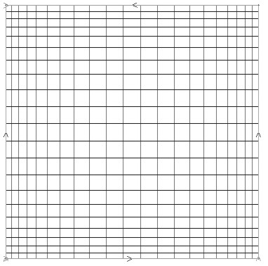 Figure 1- Cartesian Mesh.
|
| Loading the CFD Mesh Generator: |
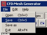
After you have opening the menu File of the CFD Mesh-Editor click in the CFD Mesh Generator.
|
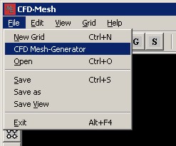 Figure 2- Loading the CFD Mesh Generator.
|
The CFD Mesh-Generator will be loaded.
|
 Figure 3-CFD Mesh-Generator.
|
| Creating a Geometry: |
| |
|
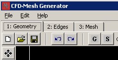 Figure 4- Geometry Tab.
|
 BackGround Grid BackGround Grid
 Snap to Grid Snap to Grid
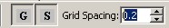
Activating these functions the mouse will just move on the drawn Grid on the window.
|
- Increases the resolution of Grid to 0.2:
|
- Click on the button to add line,
 , for the construction of the geometry of the problem. , for the construction of the geometry of the problem.
|
- Create the first Line clicking in the points (x,y)=(0.0, 0.0) and (x,y)=(0.0, 1.0). The mouse coordinates are displayed in the bottom right corner of the window.
|
- Click in the button "Zoom to Fit ",
 , to adapt the geometry to the size of the window. The final result should be similar to what is shown in the figure below. , to adapt the geometry to the size of the window. The final result should be similar to what is shown in the figure below.
|
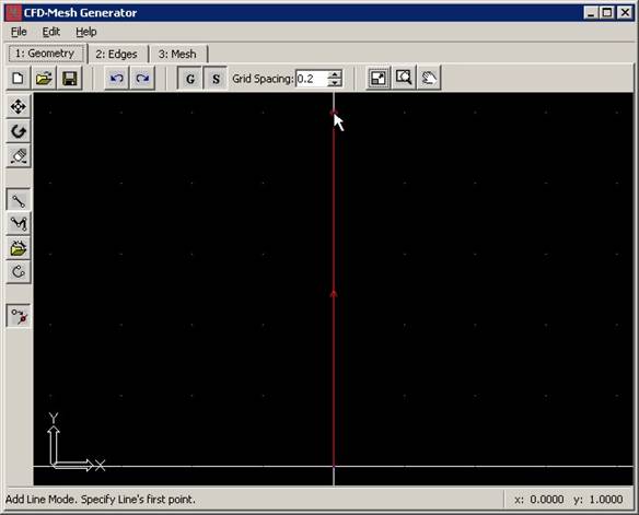
Figure 5- View after the creation of the first line.
|
- After create the following Lines:
Line 2: from (1.0, 1.0) to (0.0, 1.0)
Line 3: from (0.0, 0.0) to (1.0, 0.0)
Line 4: from (1.0, 0.0) to (1.0, 1.0)
If it is necessary, maximize your workspace for the construction of the straight line. If this is not enough, trie to configure your workspace through the button "View Mode ", . .
In the visualization mode, click twice with the left button of the mouse to increase the zoom and twice the right button to decrease the zoom. Moving the mouse with the left button you can move the geometry on the window.
The final result should be similar to what is shown in the figure below.
|
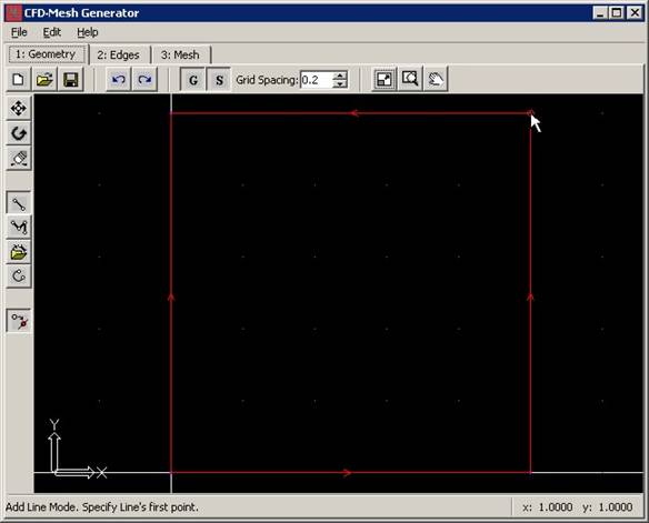 Figure 6- View after the creation of the 4 lines.
|
- Save the file in the hard disk clicking in "Save " in the main menu " File ".
|
| Creating the Computational domain |
The geometry created will serve as base for the determination of the computational domain. The computational domain must be a closed area in the space, where the mesh will be generated and where the problem will be solved.
|
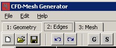
- For the definition of the computational domain select the tab "2:Edges", below to the main menu:
|
- Click on the button "Zoom to Fit ", , to maximize your workspace. You should obtain the following result:
|
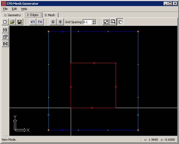 Figure 7 – Computational Domain.XXX
|
The lines in blue define the area in the space that defines the computational domain while the yellow points are the points of the mesh on the border.
Now we must make the computational domain coincide with the geometry of the problem. That is done through the projection of the borders of the computational domain on the geometry curves.
- Clicking on the button “Project Edges”,
 , on the vertical tool bar. , on the vertical tool bar.
- Click with the left button on the south border of the computational domain (the horizontal line in light blue), it will be selected and enhanced in yellow.
- Click with the left button on the straight line in red that leaves from (x,y)=(0.0, 0.0) and goes to (x,y)=(1.0, 0.0). The final result should be similar to what is shown below:
|
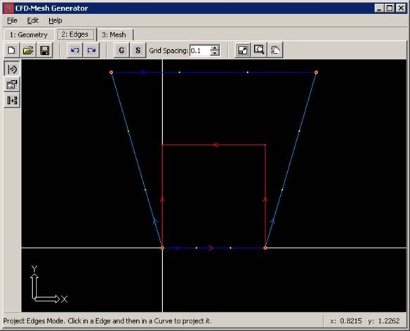 Figure 8- Projection of the south Border on one of the straight line of the geometry.
|
It should be observed that as the generated curves as the border of the domain have an orientation in the space.
In the case of the South Border the curve as the projected border have the same direction (from left to right).
In the North border we can observe that the curve is orientated from the right to the left, while the border (Edge) is orientated from the left to the right. In these situations we must projected the border in the opposite direction of the curve, as it is done below:
- Click with the left button on the North border of the Computational Domain (the horizontal line in high blue), it will be selected and enhanced in yellow.
- Click with the right button on the straight line in red that leaves from (x,y)=(0.0, 1.0) and goes to (x,y)=(1.0, 1.0).
Clicking with the right button on the curve, the software understands that the curve and the border have opposite directions and it corrects the position of the nodes on the curve automatically. The final result should be similar to the figure below:
|
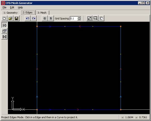 Figure 9- Projection of the second border on the geometry.
|
In case the Software have not been informed that the curve and the border have opposite direction the program would invert the direction of the border so it would have the same direction of the geometry and the result would be:
|
 Figure 10- In case of inverted projection
|
With the projection of the North and South border borders east and West ended coincident with the vertical straight line, becoming unnecessary the projection of the same ones.
Click now on the button "Edge Properties ",  , on the vertical tool bar. A panel should appear in the right part of the window. Be certified that the option " Apply to Parallel Edges " is selected, according to the figure below: , on the vertical tool bar. A panel should appear in the right part of the window. Be certified that the option " Apply to Parallel Edges " is selected, according to the figure below:
It is necessary click on the button “Zoom to Fit”,  , to maximize your workspace. , to maximize your workspace.
|
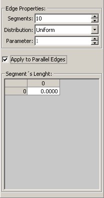 Figure 11- Tab that contends the information about the borders.
|
- Select one of the borders of the Domain.
- Increase the number of nodes to 21 with a Symmetrical Exponential distribution, with a parameter equal to 5. The border properties Tab should appear as below:
|
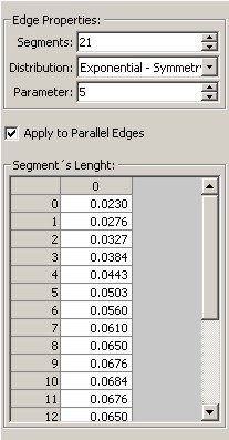 Figure 12- Tab with the right Alterations.
|
Having selected the option "Apply to Parallel Edges" the modifications done on the North border will be applied to the South borders and the modifications in the East borders will be applied on the West border.
- Repeat the operation so all the borders possess 21 nodes with a symmetrical exponential distribution with a parameter equal to 5. The final result should be similar to what is shown below:
|
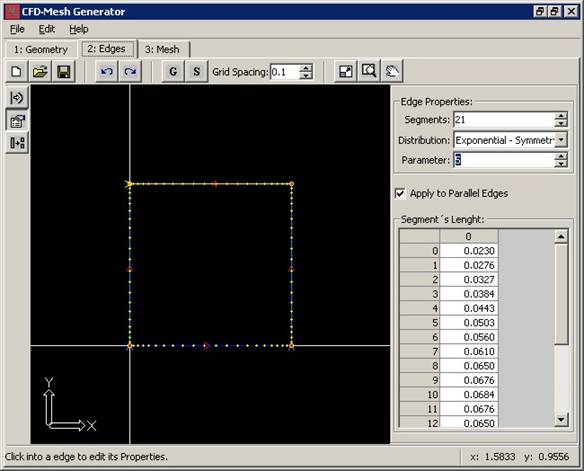 Figure 13- All the borders with 21 segments.
|
| Creating a Mesh: |
The mesh will be created on the computational domain specified in the previous item.
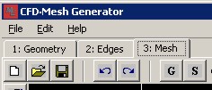
- For the creation of the mesh, select the Tab " 3: Mesh ", below of the main menu.
-
Click on the button “Zoom to Fit”, , to maximize your workspace. You can visualize the generated mesh, that should be similar the figure below:
|
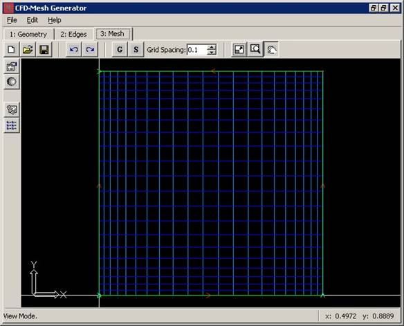 Figure 14- Mesh generated by algebraic interpolation.
|
The mesh is initially generated by an algebraic interpolation of the first order [Maliska 2004]. If no modification is necessary in the mesh, it can be exported for a file " .sdf " through the button " Export Mesh”,  , or be added to the Meshes group of the CFD Mesh-Editor through the button " Add to CFD Mesh-Editor”, . , or be added to the Meshes group of the CFD Mesh-Editor through the button " Add to CFD Mesh-Editor”, .
|