CFD Mesh-Generator:
Tutorial 02 - Mesh for simulation of flow over a car |
| |
|
|
|
| Objectives: |
The present tutorial aims to generate a 2D mesh over a car, as in Fig. 1.
In this tutorial the following facilities will be used:
- Importing of a curve defined by the user (if required)
- Discretization of the domain in blocks;
- Generation of the Mesh through Elliptic equations.
|
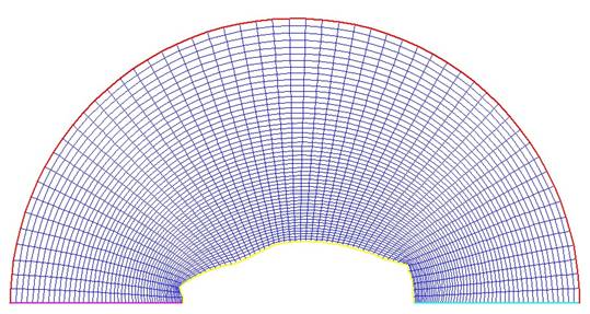 Figure 1- The mesh for simulating the flow over a car.
|
| Creating the boundaries of the computational domain: |
The computational domain is the region in the space where the grid will be generated. It is formed by boundaries given by curves created inside the application, read from files or both. For example, for the flow inside a duct, the physical boundaries of the duct form the computational domain. In the case of the flow over a car, presented in this tutorial, the computational domain is formed by the car geometry plus external boundaries that need to be created using lines and curves. Let us now follow the creation of a mesh for the flow over a car. |
|
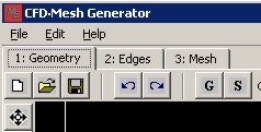 Figure 2- Geometry Tab.
|
- To assist the geometry construction, the functions "BackGround Grid ", "Snap to Grid " and " Snap to Curve Point " should be activated.
These functions can be activate by clicking on the following Buttons:
 BackGround Grid BackGround Grid
 Snap to Grid Snap to Grid
 Snap To Curve Snap To Curve
Activating these functions the mouse will just move on the drawn Grid on the window.
The "Snap to Curve" function will make the points selected by the Mouse to coincide with the extremities of the curves in case of the distance among these points are very small.
Click in the button Add Multi-Point Line from File,  , to load the file with the discretization curves of the contour of the car. , to load the file with the discretization curves of the contour of the car.
Select, one to one, the files that contain the curves and click OK. The File with the extension ".dat" contains the following information:
|
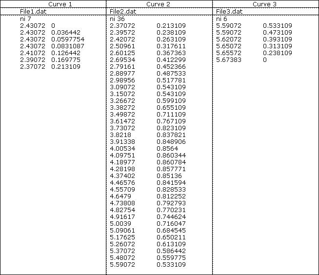 |
The first line informs the number of points of the curve and following, and next the x and y coordinates of the ni points of the curve.
For this tutorial you can create your own contour files copying the information above in three files ".dat ".
- Click on the button “Zoom to Fit”,
 , to adapt the geometry to the size of the window. The final result should be similar to the figure below: , to adapt the geometry to the size of the window. The final result should be similar to the figure below:
|
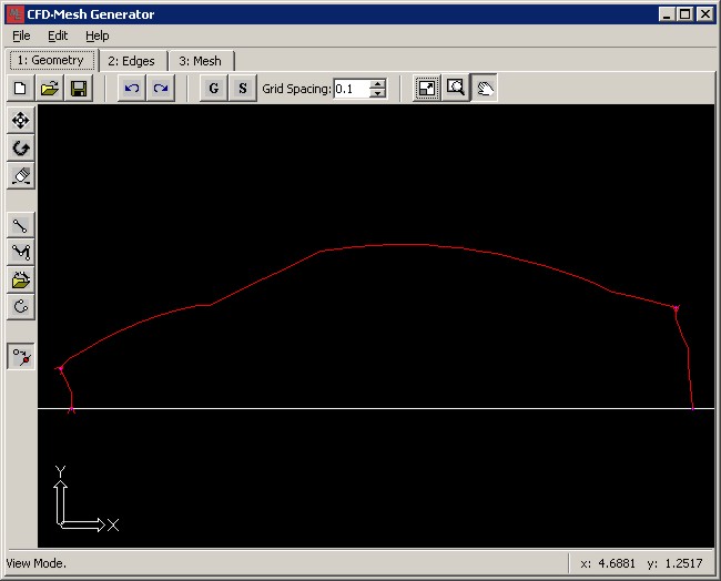 Figure 3- Configuration after the curves loading.
|
- Next, click in the button to Add line,
 , and create the following lines: , and create the following lines:
Line 1: from the beginning of the car curve to (0.0, 0.0).
Line 2: from the end of the car curve to (8.0, 0.0).
If necessary, maximize your workspace for the construction of the straight line. If this is not enough, try to configure your workspace through the button " View Mode ",  . .
In the visualization mode, click twice with the left button of the mouse to increase the zoom and twice with the right button to decrease the zoom. Moving the mouse with the left button you can move the geometry on the window.
The final result should be similar to the figure below:
|
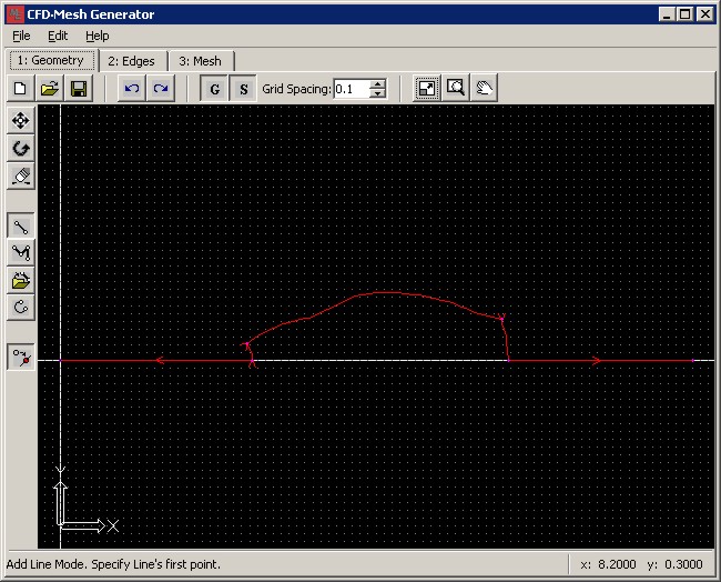 Figure 4- Configuration after the creation of the 2 lines.
|
Observe the direction of the straight lines that were created. The straight line on the left of the car has a direction from the right to the left and the straight line on the right of the car has a direction from the left to the right. Both straight lines point outside of the car surface.
- Select now the Add arch tool,
 , to complete the external contour of the domain. , to complete the external contour of the domain.
To add an arch you must specify the center, the beginning point and the final point of the arch.
Arch 1
As the center of the arch select the point (x,y)=(4.0,0.0).
As the beginning of the arch click in (x,y)=(0.0,0.0).
Maintain the CTRL key pressed so the Arch will be built in the clockwise direction.
As the final point of the arch click in (x,y)=(0.0,0.5).
Repeat this operation with the following parameters:
Arch 2:
As the center of the arch select the point (x,y)=(4.0,0.0).
As the beginning of the arch click in (x,y)=(0.0,0.5).
Maintain the CTRL key pressed so the Arch will be built in the clockwise direction.
As the final point of the arch click in (x,y)=(8.0,1.3).
Arch 3:
As the center of the arch select the point (x,y)=(4.0,0.0).
As the beginning of the arch click in (x,y)=(7.8,1.2).
Maintain the CTRL key pressed so the Arch will be built in the clockwise direction.
As the final point of the arch click in (x,y)=(8.0,0.0).
The final results should be the same as the following figure:
|
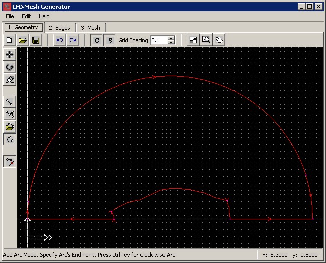 Figure 5 – Geometry Generated.
|
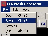
- Save the file in your hard disk clicking in "Save" in the main "menu File ".
|
| Specifying the points of the mesh at the boundaries: |
The geometry created will serve as base for the determination of the computational domain.
The computational domain should delimit a closed area in the space, where the mesh will be generated and where we will simulate the problem.
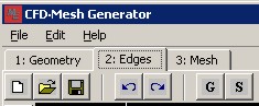
- For the definition of the computational domain select the tab " 2:Edges ", below to the main menu:
-
Click on the button "Zoom to Fit ", , to maximize your workspace. You should obtain the following result:
|
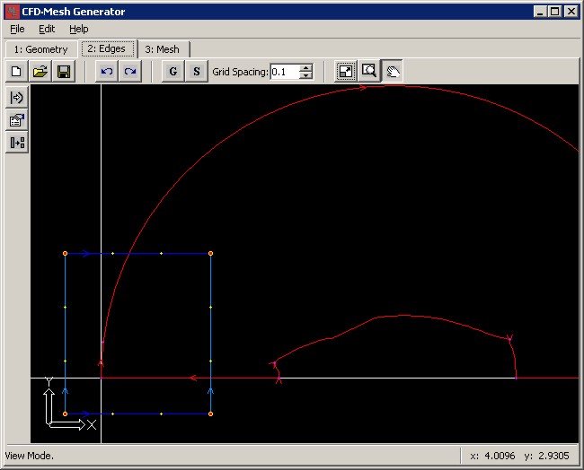 Figure 6 – Computational Domain.
|
For projection of the borders on the curves the relationship of 1x1 should be respected, the borders can be projected with only one curve.
The borders North and South, however, are being described by 3 curves (three arches for the North border and the 3 curves of contour of the automobile for the south border).
This problem is outlined through the function "Split Edges “, which divides the domain in nixnj sub-domains.
- Divide the domain in 3x1 sub-domains through the function “Split Edges”,
 , according to the figure below: , according to the figure below:
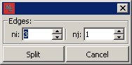
So now we have three sub-domains, according to the figure below:
|
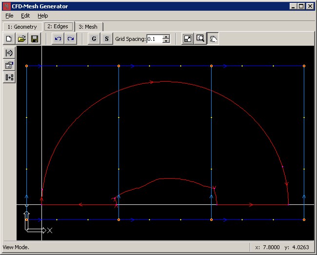 Figure 7- Sub-domain of the mesh
|
- Click on the button “Project Edges”,
 , on the tool bar. , on the tool bar.
- Click with the left button on the border West of the Computational domain (the vertical line in blue more to the left), it will be selected and enhanced in yellow.
- Click with the left button on the straight line in red that leaves the beginning of the contour of the automobile and goes to (x,y)=(0.0, 0.0). The final result should be similar to the figure below:
|
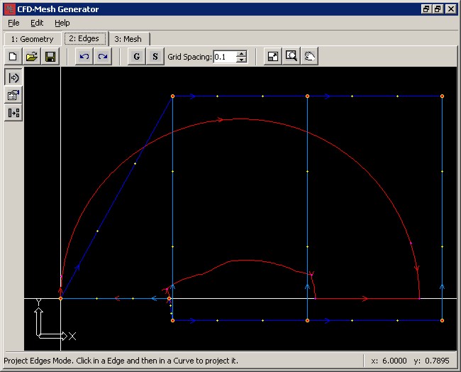 Figure 8- Projection of the Border west on one of the straight line of the geometry.
|
Project one to one the external borders on the curves in red according to the following figures. The internal borders don't need projection because they don't represent any internal contour of the domain.
|
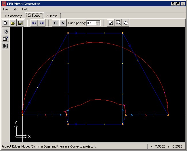 Figure 9- Projection of the east border.
|
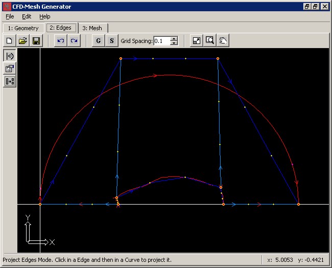 Figure 10- The south border Projection of the domain (i, j)=(1,0).
|
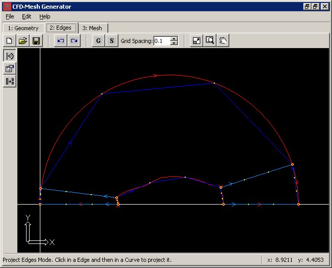 Figure 11- The north border Projection of the sub-domain (i, j)=(1,0).
|
After the borders north and south of the others Sub-domains should be projected.
- The North border of the Sub-domain (i, j)=(0,0) is projected on the Arch 1.
- The North border of the Sub-domain (i, j)=(2,0) is projected on the Arch 3.
- The South border of the Sub-domain (i, j)=(0,0) is projected on the contour curve to the left of the automobile.
- The South border of the Sub-domain (i, j)=(2,0) is projected on the contour curve to the right of the automobile.
The final result should be similar to the figure below:
|
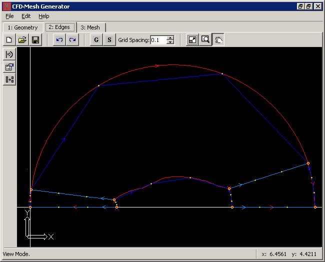
Figure 12- All the Projected borders.
|
- Click now on the button “Edge Properties”,
 , on the tool bar. A Tab should appear in the right part of the window. Be certified that the option " Apply to Parallel Edges " is selected, according to the figure below: , on the tool bar. A Tab should appear in the right part of the window. Be certified that the option " Apply to Parallel Edges " is selected, according to the figure below:
If is necessary click on the button “Zoom to Fit”, , to maximize your workspace.
|
 Figure 13- Tab contends the information about the borders.
|
- Select the border West of the domain (horizontal Border to the left).
- Increase the number of segments to 50 with an Exponential distribution, with a parameter equal to 10. The properties Tab of the border should similar to the figure below:
|
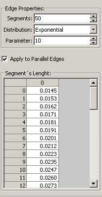 Figure 14-The Tab with the right modifications.
|
The final result should be similar to the following figure:
|
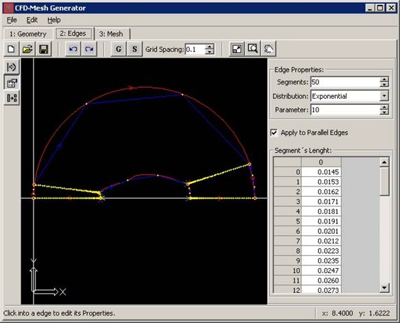
Figure 15- Border West with 50 segment, exponential distribution with parameter 10.
|
Having selected the option " Apply to Parallel Edges " the modifications done on the border West will be applied for the border East and all the internal borders.
- Select the North border of the Sub-domain (0,0).
- Increase the number of segments to 3 with an uniform distribution:
- Select the North border of the Sub-domain (1,0).
- Increase the number of segments to 47 with an uniform distribution
- Select the North border of the Sub-domain (2,0).
- Increase the number of segments to 7 with an uniform distribution
|
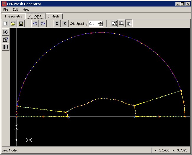 Figure 16- complete discretization of the domain contours.
|
| Creating the Mesh: |
The mesh will be created on the computational domain specified in the previous item.
- For the creation of the mesh, select the Tab " 3:Mesh ", below of the main menu.
- Click on the button “Zoom to Fit”, , to maximize your workspace. You can visualize the generated mesh, that should be similar the figure below:
|
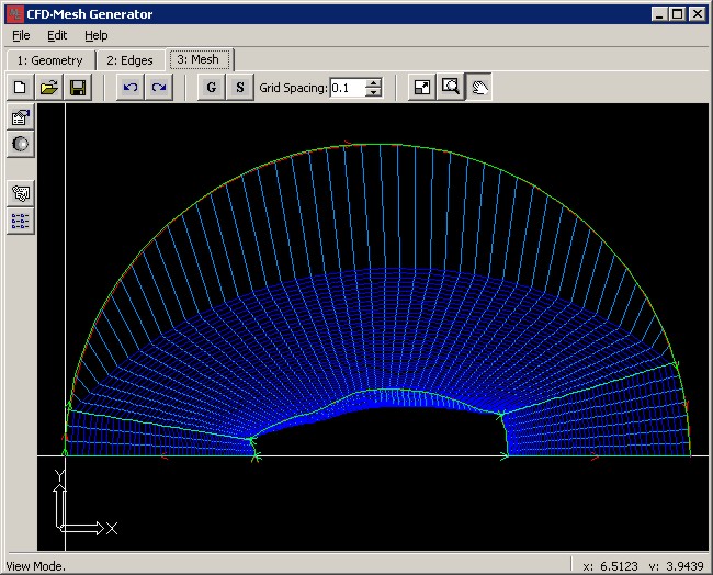 Figure 17 - Mesh generated by Algebraic interpolation.
|
The mesh is generated initially by the average of the meshes interpolated in the directions x e h.
The direction x is the one that connects the East and West boundaries and the direction h is the one that connects the North and South boundaries.
For the Mesh in consideration the best solution would be to generate a mesh interpolated in the h direction, i.e, a mesh where all the internal points would be located on the straight lines that joins the South and North border (from the surface of the car to the external curve).
- Click on the button “Block Properties”,
 , a Tab should appear on the right side of the window. , a Tab should appear on the right side of the window.
- If is necessary click on the button “Zoom to Fit”,
 , to maximize your workspace. , to maximize your workspace.
|
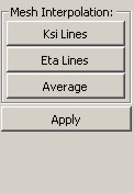 Figure 18- Tab for the control of the Mesh Interpolation.
|
- Select the Sub-domain (1,0). After in the Tab Mesh Interpolation click in "Eta Lines" and after click in "Apply". The result should be similar to the figure bellow:
|
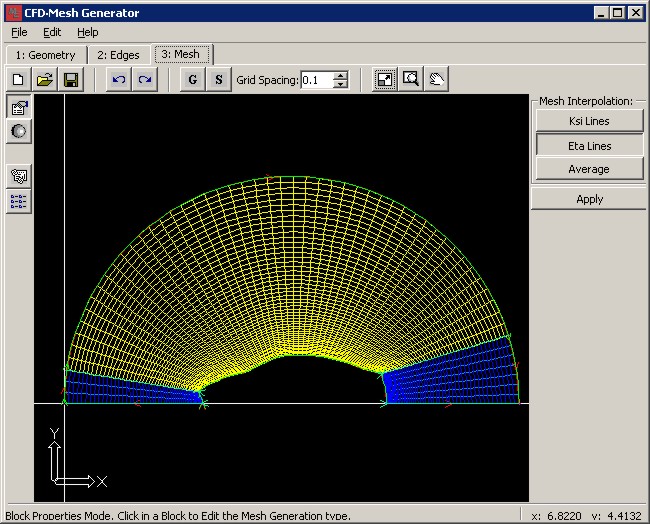 Figure 19-Sub-Domain (1,0) interpolated on the direction h.XXX
|
- Repeat the operation for the sub-domains (0,0) and (2,0). The final result should be similar to what is shown below:
|
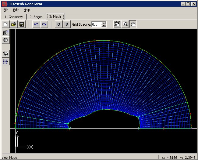 Figura 20- All the Sub-domains interpolated in the h direction.XXX
|
Analyzing the mesh on the back of the vehicle, figure 18, it is noticed that the ksi lines of the mesh presents sharp variations in direction. This problem can be corrected through the function "Smooth mesh".
|
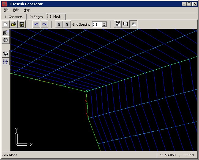 Figure 21 - Zoom of the mesh in the back of the car.
|
- Click on the button “Smooth Mesh”,
 , the following form will appear:XXX , the following form will appear:XXX
|
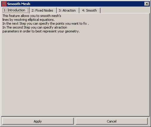
Figure 22- Form for the mesh generation through the resolution of elliptic differentials equations.
|
This form facilitates the generation of the mesh through the solution of elliptic differential equations [Maliska 2004].
It is possible to specify the parameters for generation the mesh, such as:
- Fixed points: Internal points of the mesh can be fixed, allowing that the internal contours follow some grid lines during the mesh generation.
- Attraction: The generation of the mesh through Laplace’s equation doesn't adapt very well to concave areas of the geometry, becoming necessary to specify some coordinate attraction. This is done through the specification of attraction parameters. [Maliska 2004]. The attraction parameters can only be specified for the fixed points of the mesh, created in the Tab " 2:Fixed Nodes ".
In the example in consideration no attraction parameter will be necessary since the mesh doesn't present concave areas.
- Click in the Tab " 4:Smooth ", you will have access to the parameters of the Solver, figure 20:
|
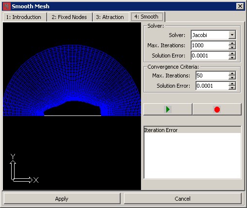
Figure 23- Setup Tab of the Solver and convergence criteria.
|
- Leave the parameters of the Solver and the convergence criteria with its default values and click in "Start Simulation",
 , and wait the end of the calculations. This stage can take some minutes depending on the velocity of the CPU processor you have on your computer. , and wait the end of the calculations. This stage can take some minutes depending on the velocity of the CPU processor you have on your computer.
- Once the problem is converged, click in the button "Apply", so the mesh will be loaded in the CFD Mesh Generator.
The final mesh should be similar to the one shown below.
|
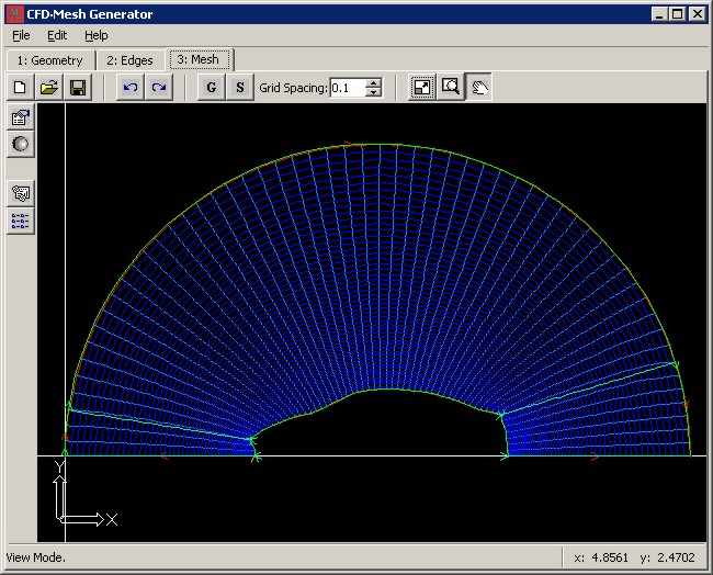
Figure 24- Mesh generated by the solution of the elliptic equations.
|
Observe that the coordinate lines on the back of the car are now smooth.
|
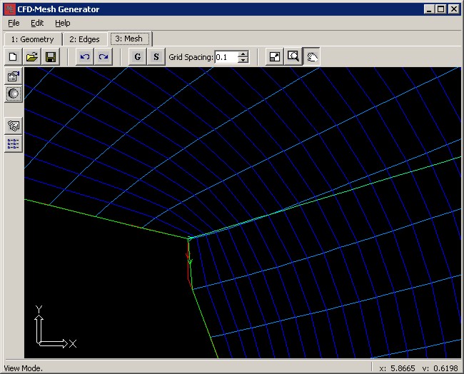
Figure 25- Mesh next to the back of the car using Lapalce’s equation for smoothing.
|
The mesh can be exported for a file " .sdf " through the button “Export Mesh”, , or can be added to the Meshes group of the CFD Mesh Editor through the button “Add to CFD Mesh-Editor”, , or can be added to the Meshes group of the CFD Mesh Editor through the button “Add to CFD Mesh-Editor”,  . .
|