| TUTORIAL CFD-STUDIO NATURAL CONVECTION IN A SQUARE CAVITY
In this problem we will use the CDS interpolation scheme and the SIMPLEC Method of (For more details about interpolation scheme, see the Scientific Manual) |
|---|


 Figure 31 – Interpolation Scheme |
||
|---|---|---|
pressure-velocity coupling. (For more details about PV Coupling methods, see Scientific Manual). On this box you can also set a sub-relaxation on the pressure. If the problem has some boundary condition where the velocity is unknown, like “open wall” and “outlet”, you can facilitate the convergence setting a Reference Pressure in the domain. This ensure that will be just one solution for the pressure field. |
||
 Figure 32 – PV Coupling Console |
||
We continue, setting a step time of 0,05s, If you desire to estimate the time interval size to be used in a certain problem you can take as base the maximum step in the allowed time if the explicit formulation was used. More details can be found in the chapter 5 of Maliska, 2004. |
||
 Figure 33 – Time Settings Console |
||
| with 20 iterations in the PV Coupling looping, and 2 in the temperature loop. |
||
 Figure 34 – Maximum Iterations Console |
||
We will use 10-5 the tolerance for the steady state for all variables. The verification is done in the two central lines of the mesh (joining S to N and W to E). |
||
 Figure 35 – Steady State Errors Console. |
||
Therefore, for our problem you will have to configure the window as in Figure 36: |
||
 Figure 36 – Numeric Parameters Console. |
||
Now click OK.
The next step is to define the solver to be used in the solution of the linear systems. In the main window click in Processor and after in Solver Settings, (Figure 37). |
||
 Figure 37 - CFD-Studio main Console |
||
and a window as the Figure 38 will appear; |
||
 Figure 38 – Solver Console |
||
The solver choice is an essential step. The direct solvers are much more precise but they need a very big memory space. The iterative solvers just work with the non null elements of the matrix, saving like this a lot of memory in the computer, but they are subject to fail with unstable linear systems (evil-conditioned matrix), because they spread mistakes according to the direction of the sweeping in the matrix The behavior of the several linear solution system methods can be found in the linear algebra text. For our problem we will use the TDMA solver. The tolerance and the maximum number of iterations must should be defined as in Figure 38. |
||
IN the main window click in Processor and then in Simulator, as shown in Figure 39. |
||
 Figure 39 – CFD-Studio main Console |
||
| You will see a window like the one in Figure 40 |
||
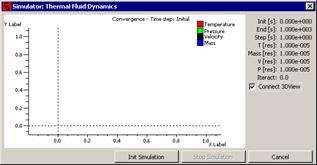
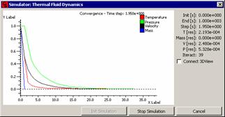
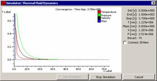
 Fig. 40 – Console do terminal de controle. |
||
In this window, you will see in the right side, the residues of the simulation. The plot shows the residues against the number of iterations. After the end of the simulation it is necessary to click in Exit to see the numerical results. You can see the images of the simulation (such as the iso-lines, pressure fields) connecting the 3D window, where you can see the simulation in real time. Only enable this function if you have a 3D video board with OpenGL support.
In the main window clicking in Processor and after in Simulator Progress and you will see a window like the one in Figure 41. |
||
 Figure 41 – Numeric Engine Console |
||
(It is not necessary to open this window now, it will open automatically as soon as the simulation begins, the same will happen with the 3D window) |
||
 |
 |
|
| Figure 42 |
Figure 43 | |
 |
 |
|
| Figure 44 |
Figure 45 | |
 |
 |
|
| Figure 46 |
Figure 47 | |
 |
 |
|
| Figure 48 |
Figure 49 | |
 |
 |
|
| Figure 50 |
Figure 51 | |
 |
 |
|
| Figure 52 | Figure 53 | |
 |
 |
|
| Figure 54 | Figure 55 | |
| © SINMEC/EMC/UFSC, 2001. | All rights reserved. |