In this tutorial, the natural convection problem inside a cavity using the CFD Studio software is studied.
The problem of natural convection explored in this tutorial, depicted in the Figure 1, consists of a square cavity with dimension LxH with a fluid initially equal to 0.5ºC, insulated in the north and south walls and with the east and west walls exposed to a temperature variation DT (west = 0ºC and east = 1ºC). The temperature variation is responsible for the movement of the fluid (see Maliska, 2004).

Figure 1 – Natural convection in a square cavity.
The first step to take after the program has been initialized is to select the problem type. In the main window click on the item Pre-Processor, then click on the item Problem Type, as shown in the Figure 2.

Fig. 2 – CFD-Studio Central Console.
It will appear a window as in the Figure 3.

Figure 3 – Console of the problem type |
       ·    The option Heat Conduction indicates that only the energy
             equation will be solved
            (Fore more details see Scientific Manual - Item 3);


       ·    The second option will solve the momentum and mass
            conservation equations;


       ·    The third option will solve the energy, momentum and
            the mass conservation equations;
|
For our problem we will use the option Fluid Flow with Heat Transfer. After selection, click OK.
The geometry definition is done in the group of elements of the pre-processor (menu pre-processor). To select click in Geometry Definition as illustrated Figure 4:

Figure 4 - CFD-Studio Central Console |
and the following window will appear (Figure 5).
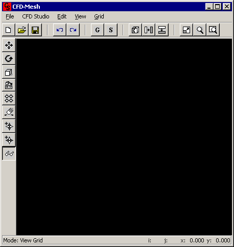
Figure 5 - CFD-Mesh Central Console |
In this stage you will create the mesh for the problem. In the item File, clicking in New Grid it will appear a window as in Figure 6:

Figure 6 – Console of mesh generation |
Now define the width (L) and the height (H) and the inclination. In this case we selected 1 meter for L and H and 90º for the inclination. The mesh will be Cartesian and it will have an uniform mesh distribution with 21 volumes in the i-direction and 21 volumes in the j-direction. Thus, your window should look the same as in Figure 7. Then click in Apply and in Close.

Figure 7 – Console of mesh generation
Don't forget to click in Set as Active Grid in the CFD-Studio item. That will define this mesh as the active mesh of our problem (Figure 8). |

Figure 8 - CFD-Mesh Central Console
After this, close this window.
The next step will be defining the initial conditions. In the main window click in Pre-Processor and in Initial Condition, as in Figure 9.

Figure 9 - CFD-Studio Central Console
|
It will appear a window as in Figure 10:

Figure 10 – Console of the Initial Condition
Here we will define the initial temperature, pressure, u and v velocity fields. In our problem the fluid will be considered at rest in t=0 with an initial constant temperature of 0.5 ºC. Thus, your window should look the same as in Figure 11. Click in Apply and in Close.
More details see Manual: Initial Conditions .

Figure 11 - Console of the Initial Condition.
Click, in the main window, in Pre-Processor and after in Boundary Conditions (Figure 12).

Figure 12 – CFD-Studio Central Console.
|
It will appear a window as in Figure 13.

Figure 13 - Console of the Boundary condition |
The Default conditions are temperature and u and v velocity fields prescribed equal to zero for all faces.
North Face:
To define the boundary conditions in the north face click in Add and in Heat Flux, as in the Figure 14.

Figure 14 – Console of the Boundary condition.
| The following window will appear: |

Figure 15 – Console of the heat flux addition
(Selecting a constant function equal to zero for this face you will be insulating the wall. It must be defined which portion of the wall have this condition. This is done defining the limits. Starting from cell 0 and ending in cell 20 means that the whole face is insulated. After this operation click in OK. The window should look the same of the Figure 16.
|

Figure 16 - Console of the Boundary condition.
South Face:
For our problem the same condition applies (Figure 17).
|

Figure 17 - Console of the Boundary condition
East Face:
For the East face, clicking in the tab East, you will see a window like the one in Figure 18.
|

Figure 18 - Console of the Boundary condition
Click in Add (you will select a condition). In our problem, Temperature need to be selected for applying the boundary condition (Figure 19). |

Figure 19 - Console of the Boundary condition
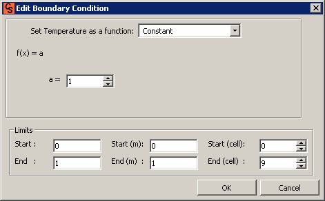
Figure 20 – Console of temperature addition in the border
We select a constant function equal to one as our temperature condition. As before, the temperature condition can be applied only in parts of the wall. This is done setting the limits. After accomplishing this operation, click OK.
The window should look the same as in Figure 21. |

Figure 21 - Console of the Boundary condition
West Face:
The same as before applies for the West face. For the natural convection problem in consideration the temperature of the west face is set to zero, as seen in Figure 23 and 24. |

Figure 22 - Console of the Boundary condition

Figure 23 – Setting the wall temperature

Figure 24 - Console of the Boundary condition
| Finally, we will now define the physical properties of the media. In the main window click in Pre-Processor and after in Physical Parameters, as in Figure 25. |

Figure 25 – CFD-Studio Central Console
| It should appear a window like the Illustration 26, because it is the Default condition. |

Figure 26 – Console of the parameter condition
| In this stage you should supply the physical properties of the media in consideration. Some materials are already pre-established, other you should enter the data. In our example we will use a pseudo fluid, with the physical properties shown in Figure 27. These parameters results in a fluid with Pr=0.71 and a Ra number based on H equals to 1214. |

Figure 27 – Console of the parameter condition
Don't forget to click in the button Apply All Cells to apply this material for all the cells, if you don't click the material gold (default) will stay as the media. Notice that each material will have a different color. |

Figure 28 – Console of the parameter condition |
More details see Manual: Physical Parameters.
Now, we will continue to setup the problem, specifying parameters of the numerical simulation.
|