| CFD Studio |
|||
CFD Problem Wizard |
|||
| Creating a problem with the CFD Problem Wizard | |||
PATH: On PROBLEM menu, click NEW, and choose CFD Problem Wizard as in the Figure 1. This option allows assisting the user, indicating the several necessary steps for the creation of a numeric problem in CFD. These steps are: mesh generation of the simulation, boundary conditions, numeric parameters of simulation and the simulation. |
|||
|
|||
| With this will appear the following window (Figure 2). Informing about the Wizard 8 steps. | |||
 Figure 2 – Wizard 8 steps information |
|||
| Then click OK to proceed or CLOSE WIZARD to leave the CFD Problem Wizard. OBS: Always remember to give APPLY in the configuration windows to add the data to the problem, otherwise the same ones won't be accomplished. |
|||
 Figure 3 – Step 1– Problem Type |
|||
The first step is to choose the problem type to be solved (Figure 4): |
|||
 Figure 4 – Problem Type |
|||
The second step (Figure 5) is the discretization of the domain (Figure 5). The CFD-Mesh software can create, edit or open an existing mesh, to be used in the CFD Studio (Tutorial CFD-Mesh). |
|||
 Figure 5 – Step 2– CFD-Mesh.  Figure 5.b –CFD-Mesh Interface – SET AS ACTIVE GRID selected. |
|||
In this step will be setup the initial conditions of the problem (Figure 6). |
|||
 Figure 6 – Step 3 – Initial Conditions |
|||
In the following window (Figure 7) will be setup the initial conditions of the problem: temperature, velocity u and v, and pressure. The user can determine only one value for the initial field of the variables, or to impose a field already pre-defined, starting from the reading of a data file (file of the type " * .dat ": file ASCII in the format i x j of values – values table). The same can be made imposing an initial condition, starting from the last simulate data (i.e.: to re-begin a simulation interrupted, it just impose as initial condition the last results obtained). More details see Manual: Initial Conditions and Tutorial: CFD Studio - Natural Convection. |
|||
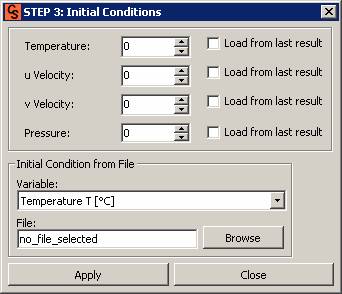 Figure 7 – Initial Conditions Setup |
|||
In this step the boundary conditions will be selected in each face of the mesh (Figure 8). |
|||
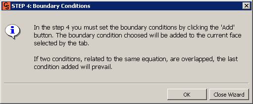 Figure 8 – Step 4 – Boundary Conditions |
|||
In the following window (Figure 9) the conditions will be given for the boundary North, South, East and West of the simulation mesh. These boundary conditions can be temperatures or prescribed velocities, inlet or outlet conditions, etc. More details see Manual: Boundary Conditions and Tutorial: CFD Studio - Natural Convection . |
|||
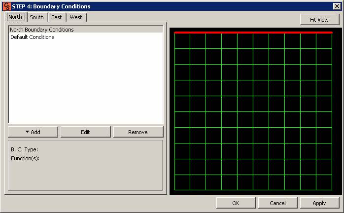 Figure 9 – Boundary Conditions Setup |
|||
In this step (Figure 10) will be chosen the material type and its properties can be edit (Figure 11). More details see Manual: Physical Parameters and Tutorial: CFD Studio - Natural Convection. |
|||
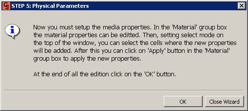 Figure 10 – Step 5 – Physical parameters 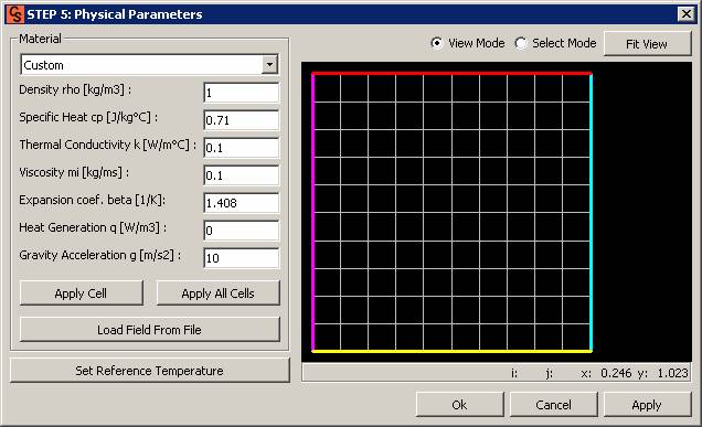 Figure 11 – Physical parameters Setup |
|||
In this step (Figure 12) will be chosen the interpolation scheme, the Pressure-velocity coupling type, the convergence criteria and the iteration error (Figure 13). More details see Tutorial: CFD Studio - Natural Cnvection. |
|||
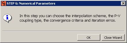 Figure 12 – Step 6 – Numeric Parameters  Fig. 13 – Setup dos Parâmetros Numéricos. |
|||
| |
|||
In this step (Figure 14) will be chosen which solver will be used to solve the linear systems (Figure 15). |
|||
 Fig. 14 – Step 7 – Solver. |
|||
You can also choose the tolerance of the solver and the iteration limit. More details see Tutorial: CFD Studio - Natural Convection. |
|||
 Fig. 15 – Solver Setup |
|||
In the last step (Figure 16) the simulation of the generated problem will be accomplished. |
|||
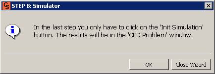 Fig. 16 – Step 8 – Simulator. |
|||
In the simulation window (Figure 17) will be shown the final and initial time, the step, the temperature, mass, velocity and pressure error and the iterations number. The mesh can still be visualized in 3D during the simulation, selecting CONNECT 3DVIEW (only for equipments with graphic acceleration, OpenGL support). More details see Tutorial: CFD Studio - Natural Convection. IMPORTANT: The iterative visualization of the results in the post-process window (window 3D) can only be accomplished with the use of a graphic card with support to OpenGL. |
|||
 Figure 17 – Simulation convergence view. |
|||

| © SINMEC/EMC/UFSC, 2001. | All rights reserved. |